 When combining p-values in a meta-analysis framework there are many different methods we can apply based upon where the p-values come from and what their relationship is. The most well known methods being Fisher’s Method and Stouffer’s.
So I thought I would add one more out of fun and because why not; The Bayesian P-Value method!
So this is how….
Turns out that thanks to Selke, Bayarri & Berger we have this cute little formula to turn p-values into the posterior probability of H0 that arises from use of the Bayes factor together with the assumption that H0 and H1 have equal prior probabilities of 1/2.
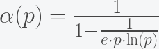
Cool, uh? The “only” caveat is that this formula just works for p-values lower or equal than 1/e ~ 0.36 so for greater p-values we might be out of luck but, considering that usually we want to combine small p-values, this limitation might not be much of a problem in many situations.
All right, so now that we have turned the p-values into Bayesian probabilities we can use a little of Naive Bayes to combine these probabilities together into one to then use the inverse of our little formula above to recover the p-value that would correspond to such Bayesian probability.
Example
Let’s say we have three p-values coming from three identical experiments with results: 0.05, 0.1 & 0.2. Now let’s apply the previous steps depicted in the following diagram and in this code.

These are the results of combining these three p-values with three different methods:
| Method | P-Values Set | Naïve Bayes | Combined P-Value |
|---|---|---|---|
| Fisher’s | 0.05, 0.1, 0.2 | – | 0.0317663 |
| Stouffer’s | 0.05, 0.1, 0.2 | – | 0.01479742 |
| Bayesian P-Value | 0.05, 0.1, 0.2 | 0.1823287 | 0.02132706 |
And as we can see the result for the Bayesian P-Value falls nearly right in the middle of Fisher’s and Stouffer’s results in this example. Oh, well.

Interesting and i would say useful. The main theme here seems to be either a statistical test or more generaly a functional which provides an appropriate combination or more correctly translation into a probability (or sth else)
In this respect you might be interested in the axiomatic characterisation of the entropy method and functional and the least squares method and functional by Imre Csiszar
Why Least squares and Maximum Entopy? An axiomatic approach to inference for Linear Inverse Problems, Imre Csiszar 1991, Annals of Statistics
It turns out that the domain of application itself, can determine the appropriate functional to some extend.
PS the formula to transform a
p-valueinto a probability contains the formula for the information content of a probability (partition) i.eI(p) = -p ln(p)Interesting, thanks for the link Nikos!
Note (in the Csiszar paper i linked) that when the domain is the positive real line ie
R+, the functional is the entropic functional employing the logarithm (which is defined only for positive numbers) or in other words the logarithm in the functional determines the underlying domain to beR+. It is good to study these relations between functionals and domainsIn a sense, the functional should be such that describes or captures adequately the underlying domain. So your underlying domain is
R+? Then your functional should reflect this condition, by employing a logarithm. This is one reason why logarithms and the Shannon /Kullback-Leibler functionals are ubiquitous in probabilistic settingsEven more clearly, i want to describe R+, the logarithm function itself in fact describes R+. More correctly it describes adequately and uniquely (under some regularity conditons) the maping
f: R+ -> R. This is a basic idea of, for example, algebraic geometry. Using, this time, polynomial functionals, to describe certain spaces and subspaces. What is stated here is simlar to that.Continuing what i stated previously, note the the following. On what is already stated the following functions are in fact not equivalent
1.
x2.
exp(ln(x))3.
ln(exp(x))1) can be defined over either the whole
Ror justR+, whereas 2) is defined only inR+, and 3) overR. So they dont represent the exact same function (although usualy taken to), since the domain of application or definition is part of the function.Furthermore one could be surprised how manipulating things as the above can be used in areas like dimensional regularisation of quantum mechanics. For example dimensional regularisation or regularisation by cutoff effectively substritutes functions with other partialy equivalent functions in order to get at a finite result.